Search
Close this search box.

Algorithmic Robotics and Motion Planning, Fall 2023–2024

source: manh.com

Fall 2023/2024, 0368-4010-01

Instructor: Dan Halperin, [email protected]
Office hours by appointment

Course hours: Monday, 16:00-19:00

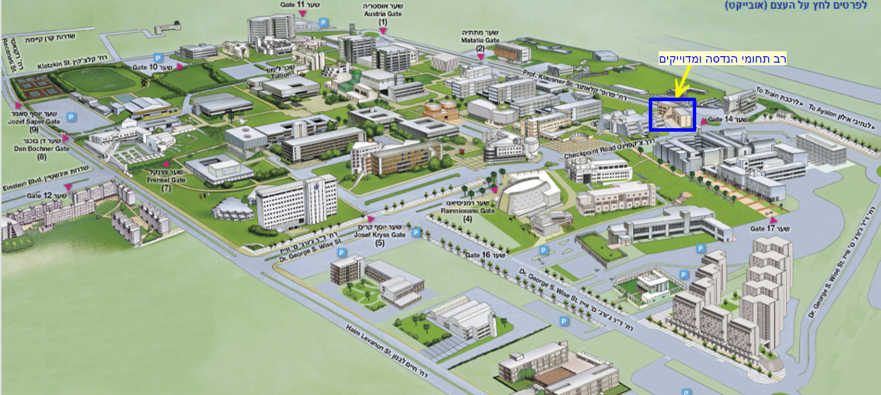
Location: Multi-disciplinary center 315 Link to map

Teaching assistant: Michal Kleinbort, [email protected]
Office hours by appointment

Recitations: Monday, 19:00-20:00

Location: Holtzblatt auditorium 007

Grader and software helpdesk: Michael Bilevich, [email protected]

Software helpdesk: Yuval Rubins, Mondays by appointment ([email protected])

source: LA times

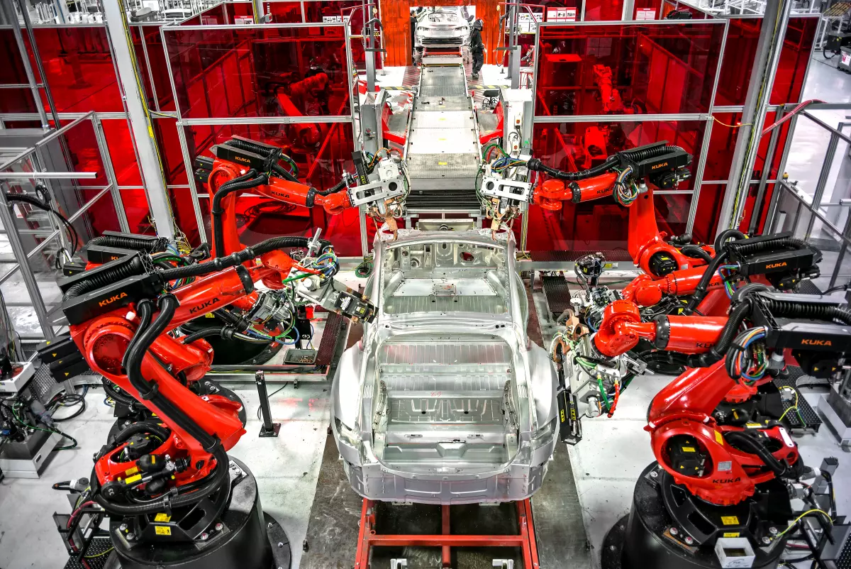
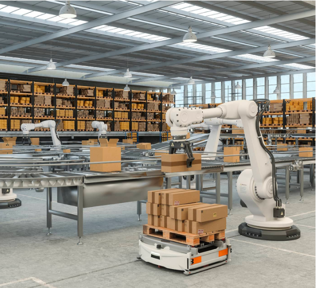
The recent years have seen an outburst of new robotic applications and robot designs in medicine, entertainment, security and manufacturing to mention just a few

areas. Novel applications require ever more sophisticated algorithms. In the course, we shall cover computational and algorithmic aspects of robotics with an emphasis on motion planning.

The motion-planning problem is a key problem in robotics. The goal is to plan a valid motion path for a robot (or any other mobile object for that matter) within a given environment, while avoiding collision with obstacles. The scope of the motion-planning problem is not restricted to robotics, and it arises naturally in different and diverse domains, including molecular biology, computer graphics, computer-aided design and industrial automation. Moreover, techniques that were originally developed to solve motion-planning problems have often found manifold applications.

The topics that will be covered include (as time permits):

source: Inventooly.com
  • A brief tour of algorithmic problems in robotics
  • The configuration space approach and the connection between motion planning and geometric arrangements
  • Minkowski sums; exact and efficient solution to translational motion planning in the plane
  • Translation and rotation in the plane; translational motion of polyhedra in space
  • Sampling-based motion planning
  • Collision detection and nearest-neighbor search
  • Path quality: shortest paths, high clearance paths, other quality measures, multi-objective optimization
  • Multi-robot motion planning: Exact motion planning for large fleets of robots—the labeled vs. unlabeled case; sampling based planners for multi-robot motion planning and the tensor product—dRRT, dRRT*

Prerequisites

The course is geared towards graduate students in computer science. Third-year undergrads are welcome; in particular, the following courses are assumed: Algorithms, Data structures, Software1.


The final grade

50% Homework assignments + 50% final project;

Link to bibliography


Assignments

  • Assignment no. 1 (pdf), due: 22.1.24, additional information: E1.1, E1.2 (Discopygal Starter), E1.3b
  • Assignment no. 2 (pdf), due: 12.2.24, additional information: E2.4
  • Assignment no.3 (pdf), due: 26.2.24, additional information: E3.1
  • Assignment no.4 (pdf), due: 11.3.24, additional information: E4
  • The final project (pdf), due: 16.6.24

Submission Guidelines

  • Each question will have its own Moodle submission page.
  • For theoretical questions, please submit a single PDF file, named: qX_IDNUM.pdf or qX_IDNUM1_IDNUM2.pdf (if submission in pairs is allowed). Example: q3_123456789.pdf.
  • When submission in pairs is allowed, only one of the students should submit the work. The grade will be updated for both students regardless.
  • While Python is preferred, code assignments can be written in any (conventional) programming language you’d like. Please contact us if you intend on using any language that is not Python, C, C++, C# or Java.
  • Code submissions should be in a single tarball (*.zip or *.tar.gz) with the same convention like PDFs, i.e., qX_IDNUM.tar.gz.
  • Important: For the code assignments, please submit a single tar/zip file, named q{num}_{id1}_{id2…}.zip. For example, for the second questions: q2_123456789_987654321.zip.
    That zip should have only one *.py file, containing the entire code of your solver. Any other files (like README, scenes, etc.) are fine.
    Also please make sure that loading that single python file into the solver_viewer tool works correctly.

Reinstallation of Discopygal

Run the following commands in your shell:

  1. pip uninstall discopygal-taucgl-starter discopygal-taucgl cgalpy
  2. pip install https://www.cgl.cs.tau.ac.il/wp-content/uploads/2024/02/discopygal_taucgl-1.0.7-py3-none-any.whl

Guest Lectures

  • Ken Goldberg, UC Berkeley, 29.1.24: The new wave in grasping
  • Kiril Solovey, Technion, 5.2.24: Introduction to robot control
  • Steven M. LaValle, Oulu University, Finland, 19.2.24: From RRTs to the path to minimalism
  • Yahav Avigal, Jacobi Robotics and UC Berkeley, 4.3.24: The academia2real gap in robotics

Mini talks by students

Cancelled due to the shortening of the semester


The course summary (week by week), the slides and additional material are uploaded to Moodle

No need to install a new version of Discopygal. (If haven’t install yet, install the one from the course’s web page)

Basic PRM solver to use as a base PRM solver (is also already in the package): prm

Exercise 4.1

Scenes to solve: ex4.1

Exercise 4.2

Scenes to solve: ex4.2

For this Assignment reinstall Discopygal to the new version: https://www.cgl.cs.tau.ac.il/wp-content/uploads/2024/02/discopygal_taucgl-1.0.7-py3-none-any.whl

See documentation https://www.cs.tau.ac.il/~cgl/discopygal/docs/code/geometry_utils/collision_detection.html about the collision detection functions of rod and how to use them.

In order to set the angle of the rod and decide the direction of rotation (clockwise or counter-clockwise) – add to the ‘data’ dict of each PathPoint in the solution path “theta” for the angle and “clockwise” (True/False) to decide if the rotation from this point to the next will be clockwise or counter-clockwise.

Exercise 3.1

Example scenes to solve for rod: rod_scenes

BasicRodPRM Solver (is also included in the package): prm_rod

Using Discopygal

Documentation about Discopygal package is found at: https://www.cs.tau.ac.il/~cgl/discopygal/docs/tutorials/getting_started.html

Follow the installation and usage instructions.

The whl file of the package: discopygal_taucgl-1.0.6-py3-none-any.whl

If you already have (an older version of) DiscoPygal installed (and you should), follow the reinstall guide.

Homework Specific Info

  • E2.4:
    Use your solver on the following scenes: narrow_gates.zipMake sure you understand how to create and modify arrangements in CGALPY (see this tutorial).
    Use the collision detection class to construct the arrangement (which is given in the cspace argument, e.g., collision_detection.cspace),
    then add vertical walls to create the vertical trapezoidal decomposition (this is only a suggestion, any valid decomposition to simpler parts will be accepted).
    After making the decomposition, construct a connectivity graph that connects each neighboring free (or semi-free) regions. Use this graph for (optimal) path planning.You may visualize your constructed arrangement by implementing the “def get_arrangement(self): Arrangement_2” method of your solver class.
    If you do so, in the solver_viewer executable, press on the “View arrangement” button: Hint: nodes in the connectivity graph may correspond to vertices, halfedges and faces in the arrangement.

Exercise 1.3b

It is possible to graphically  draw a polygon with the functions for cgalpy: Polygon.draw, Polygon_with_holes.draw.

To use the draw function reinstall a new version of discopygal package. In your environment run:

  1. pip uninstall discopygal-taucgl-starter cgalpy
  2. pip install https://www.cgl.cs.tau.ac.il/wp-content/uploads/2023/08/discopygal_taucgl_starter-1.0.6-py3-none-any.whl (takes a long time)

Code example:

import CGALPY_epec as GALPY
Point=CGALPY.Ker.Point_2
p1 = Point(0,1)
p2 = Point(1,0)
p3 = Point(0,0)
p = CGALPY.Pol2.Polygon_2([p1,p2,p3])


CGALPY.Pol2.draw(p)


Exercise 1.2

Documentation about Discopygal package is found at: https://www.cs.tau.ac.il/~cgl/discopygal/docs/tutorials/getting_started.html

Follow the installation and usage instructions.

The whl file of the package: discopygal_taucgl_starter-1.0.5-py3-none-any.whl

Install the package, be able to use it and run solver_viewer and understand how to write a solver (be helped by the example of Random Solver) Also attached here these examples as files: discopygal_starter_examples.zip

The scene to solve: coffee_shop.json

Exercise 1.1

General

  • Name the archive either oskar.zip or oskar.tar.gz
  • Name the basename (the filename without the extension) of the program file oskar
    • If you develop C++ the file should be oskar.cpp
    • If you develop Python the file should be oskar.py
    • etc…

Input

sx sy sz dx dy dz filename

The program should accept 7 arguments on the command line:

  • The source location of the robot (sx sy sz), followed by the destination of the robot (dx dy dz), followed by the name of the file that contains the description of the obstacle (filename).
  • Each location is a vector of three integer values specifying the x, y, and z coordinates of the robot center.
  • A valid input file starts with the x, y, and z dimensions (in that order) of the puzzle, followed by three matrices representing the xy-, yz-, and zx- faces; 0 represents a free location and 1 represents a forbidden location.
    • The entry in row i >= 0 and column j >= 0 in the xy-matrix represents the value for x=j and y=i. The same holds for the two other matrices.
  • The dimensions of the standard Oskar puzzle are 11, 11, 11. One pair of source and destination locations is (3, 7, 7) and (5, 1, 1).
  • You can obtain the file that contains the three (11 x 11) matrices of the standard Oskar puzzle here.

Output

The program should export the result to the standard output. The output format must be identical to the format of the verifier (see below). It consists of three lines.

The first and second lines contain the start and end positions, respectively. Each position consists of three integer values separated by spaces.

The third line contains a sequence of commands separated by spaces. Applying these commands to the robot should move it from the source location to the destination location without passing through forbidden locations. A command is encoded as follows:

  • 0 — move one unit along the x-axis in the positive direction
  • 1 — move one unit along the x-axis in the negative direction
  • 2 — move one unit along the y-axis in the positive direction
  • 3 — move one unit along the y-axis in the negative direction
  • 4 — move one unit along the z-axis in the positive direction
  • 5 — move one unit along the z-axis in the negative direction

Oskar verifier and simulator

In the following website you can verify your solution and visualize the simulation: http://www.cs.tau.ac.il/~michaelmoshe/oskar-visualization/

You can rotate the viewport by clicking and dragging the left mouse button, and zoom in and out with the mouse scroll wheel.

On the top left corner of the simulator there are three input fields which have the following format (from top to bottom):

  • Start position (e.g. 3 7 7)
  • End position (e.g. 1 7 9)
  • Command sequence (e.g. 4 4 1 1)

After entering the input you can press the play button on the bottom of the simulator to view the simulation in action! You can also press the “Verify” button to verify your input without playing the animation (and get the result immediately).

There is a log message on the bottom left corner, which displays an error/success message or the verifier/simulation.

Books:

  • S.M. LaValle, Planning Algorithms, Cambridge University Press, 2006 link
  • J.-C. Latombe, Robot Motion Planning, Kluwer Academic Publishers, 1991 (then Springer)
  • Kevin Lynch and Frank Park, Modern Robotics, Cambridge University Press, 2017 link
  • H. Choset, K.M. Lynch, S. Hutchinson, G. Kantor, W. Burgard, L.E. Kavraki, and S. Thrun, Principles of Robot Motion: Theory, Algorithms, and Implementations, The MIT Press, 2005
    in particular Chapter 7
  • M. de Berg, O. Cheong, M. van Kreveld, and M. Overmars, Computational Geometry: Algorithms and Applications, 3rd Edition, Springer, 2008

Survey papers:

Yair Oz - Webcreator

Contact

Skip to content