Given a polygon \(W\), a depth sensor placed at point \(p=(x,y)\) inside \(W\) and oriented in direction \(\theta\) measures the distance \(d=h(x,y,\theta)\) between \(p\) and the closest point on the boundary of \(W\) along a ray emanating from \(p\) in direction \(Θ\). We study the following problem: Give a polygon \(W\), possibly with holes, with n vertices, preprocess it such that given a query real value \(d \geq 0\), one can efficiently compute the preimage \(h^{−1}(d)\), namely determine all the possible poses (positions and orientations) of a depth sensor placed in \(W\) that would yield the reading \(d\). We employ a decomposition of \(W \times S^1\), which is an extension of the celebrated trapezoidal decomposition, and which we call rotational trapezoidal decomposition and present an efficient data structure, which computes the preimage in an output-sensitive fashion relative to this decomposition: if \(k\) cells of the decomposition contribute to the final result, we will report them in \(O(k+1)\) time, after \(O(n^2 \log n)\) preprocessing time and using \(O(n^2)\) storage space. We also analyze the shape of the projection of the preimage onto the polygon \(W\); this projection describes the portion of \(W\) where the sensor could have been placed. Furthermore, we obtain analogous results for the more useful case (narrowing down the set of possible poses), where the sensor performs two depth measurement from the same point \(p\), one in direction \(\theta\) and the other in direction \(\theta+\pi\). While localizations problems in robotics are often carried out by exploring the full visibility polygon of a sensor placed at a fixed point of the environment, the approach that we propose here opens the door to sufficing with only few depth measurements, which is advantageous as it allows for usage of inexpensive sensors and could also lead to savings in storage and communication costs.
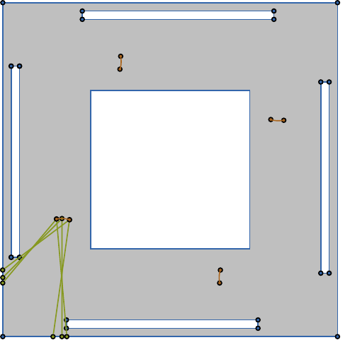
More Examples
|
|
|
|
|
|
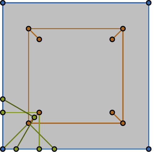
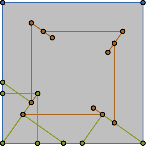
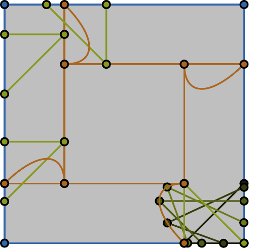
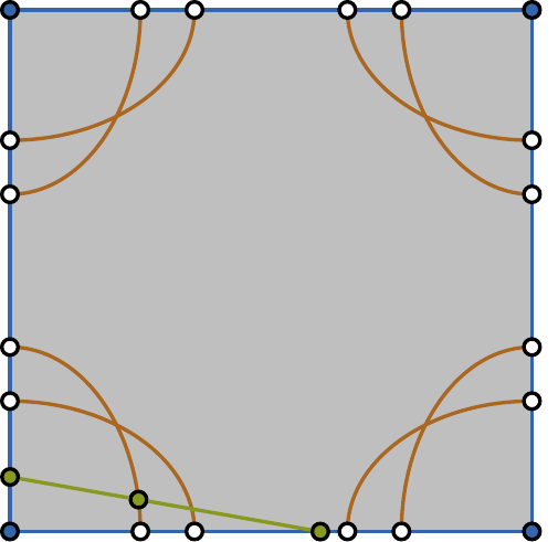
| The free space is filled with a light-gray color. The boundary of the free space is drawn with blue segments. Orange curves comprise all the possible locations of the sensor. A pair of green segments with a common endpoint shows a witness | ||||