Search
Close this search box.

Algorithmic Robotics and Motion Planning, Fall 2019–2020

Fall 2019/2020, 0368-4010-01

Course hours: Monday, 16:00-19:00

Recitations: Monday, 19:00-20:00

Location: Sherman 003

Instructor: Dan Halperin, danha AT post tau ac il
Office hours by appointment

Teaching assistant: Michal Kleinbort, balasmic at post tau ac il
Office hours by appointment

Grader: Yair Karin, yair dot krn at gmail com

Software helpdesk: Nir Goren, nirgoren at mail tau ac il, Office hours by appointment


The recent years have seen an outburst of new robotic applications and robot designs in medicine, entertainment, security and manufacturing to mention just a few areas. Novel applications require ever more sophisticated algorithms. In the course, we shall cover computational and algorithmic aspects of robotics with an emphasis on motion planning.

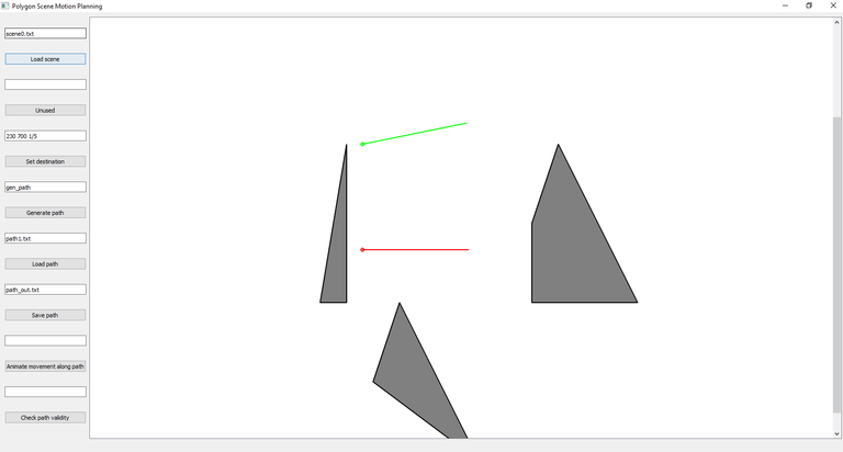
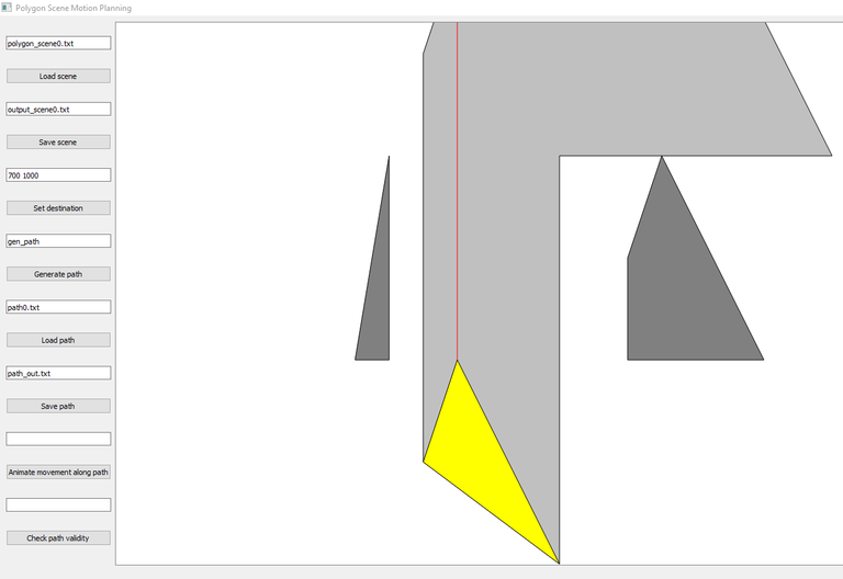
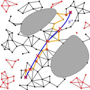
The motion-planning problem is a key problem in robotics. The goal is to plan a valid motion path for a robot (or any other mobile object for that matter) within a given environment, while avoiding collision with obstacles. The scope of the motion-planning problem is not restricted to robotics, and it arises naturally in different and diverse domains, including molecular biology, computer graphics, computer-aided design and industrial automation. Moreover, techniques that were originally developed to solve motion-planning problems have often found manifold applications.

The topics that will be covered include (as time permits):

  • A brief tour of algorithmic problems in robotics
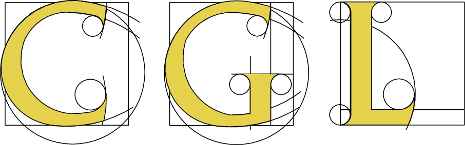
  • The configuration space approach and the connection between motion planning and geometric arrangements
  • Minkowski sums; exact and efficient solution to translational motion planning in the plane
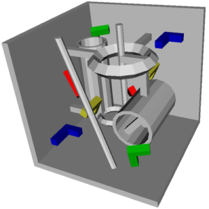
  • Translation and rotation in the plane; translational motion of polyhedra in space
  • Sampling-based motion planning
  • Collision detection and nearest-neighbor search
  • Path quality: shortest paths, high clearance paths, other quality measures, multi-objective optimization
  • Direct and inverse kinematics: from industrial manipulators to proteins
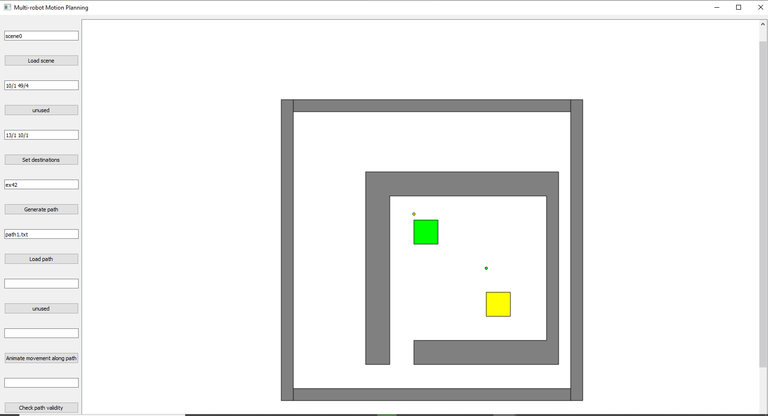
  • Multi-robot motion planning

Prerequisites 

The course is geared towards graduate students in computer science. Third-year undergrads are welcome; in particular, the following courses are assumed: Algorithms, Data structures, Software1.


The final grade

Homework assignments (40%), brief talk in class on a topic of the student’s choice (subject to approval) (10%), final project (50%).


A short bibliography:  

books and surveys


Assignments

  1. Assignment no. 1 file , due: November 11th, 2019, additional information.
  2. Assignment no. 2 file , due: December 9th December 2nd, 2019, additional information.
  3. Assignment no. 3 file , due: December 31st , 2019, additional information. Notice that Ex. 3.4 is a theory exercise.
  4. Assignment no. 4 file , due: January 23rd, 2020, Ex. 4.4 is due January 16th 2020, additional information.
The final project file , due: March 6th, 2020

Guest Lectures

  • Guy Hoffmnan, Cornell, 23.12.19: Designing Robots and Designing with Robots: New Strategies for an Automated Workplace
  • Ilana  Nisky, BGU, 6.1.20: Haptics for the Benefit of Human Health [slides]
  • Aviv Tamar, Technion, 2.12.19: Machine Learning in Robotics
  • Lior Zalmanson, TAU, 25.11.19: Trekking the Uncanny Valley — Why Robots Should Look Like Robots?
Due to shortage in teaching time for the regular course material, one invited lecture was canceled; it will be given as part of the CG seminar in the second semester.

Mini talks by students

  • Golan Levy, 4.11.19: How Do Robots See? On Lidar and Other Detection Systems [slides]
  • Itay Yehuda, 11.11.19:  Minimizing Radioactive Influence, or How to Balance Length and Clearance [slides]
  • Tom Verbin, 18.11.19:  Rotations in Space with Quaternions [slides]
  • Dror Dayan and Nir Goren, 18.11.19: Efficient Algorithms for Optimal Perimeter Guarding [slides]
  • Dor Israeli, 9.12.19: Friendly Introduction to Robotic Estimations Using Kalman Filters [slides]
  • Adar Gutman, 9.12.19: Complexity of the Minimum Constraint Removal Problem [slides]
  • Tal Eisenberg, 9.12.19: Neural Prosthetics: From Brain Activity to Robotic Motion and Back
  • Inbar Ben david, 16.12.19: A Brief Introduction to ROS
  • Or Yarinitzky and Liran Zusman, 16.12.19: Robotics StackExchange: Efficient, High-Quality Stack Rearrangement
  • Or Perel, 16.12.19: An Arm and a Leg: Humanoid Robots Design
  • Yossi Khayet, 23.12.19: Robots and Chess: from The Turk to beating Grandmasters
  • David Krongauz, 23.12.19: Foraging in Swarm Robotics: Inspired by Ants, Implemented by Robots
  • Guy Korol, 30.12.19: Soft Robotics: Designing Robotic Actuators Made from Flexible Materials [slides]
  • Harel Oshri, 30.12.19: Computational Interlocking Furniture Assembly
  • Nadav Ostrovsky, 30.12.19: Collisions as Information Source in Multi-Robot Systems
  • Nave Tal, 30.12.19: Tabletop Rearrangements with Overhead Grasps [slides]
  • Netanel Fried, 30.12.19: Using Simple Robots in Challenging Terrains
  • Tomer Davidor, 30.12.19: Using Game Theory for Autonomous Race Cars
  • Eitan Niv, 13.1.20: Locomotion Algorithms for Snake Robots
  • Lana Salameh, 13.1.20: Nano robotics – Automatic Planning of Nanoparticles Assembly Tasks
  • Doron Kopit, 13.1.20: Controlling a Swarm: Centralized vs Decentralized
  • Dan Flomin, 13.1.20: Tasty Robots: Capsule Robotics in Gastroenterology Medicine
  • Abed Khateeb, 20.1.20: Low-cost Aggressive Off-Road Autonomous Driving

Course summary

  • 28.10.19 
    Introduction [pdf]
    Recitation 1: Intersection of half-planes [pdf]
  • 4.11.19 
    Robots with 2 dofs and two-dimensional state spaces
    Disc among discs [slides], proof of the combinatorial bound [pdf]
    Minkowski sums and transnational motion planning [slides, up till Slide #15]
    Recitation 2: Plane sweep for line segment intersection. [pdf, the slides are by Marc van Kreveld]
  • 11.11.19 
    Minkowski sums, continued [slides, #15-39]
    Motion planning and geometric arrangements, general exposition [slides, up till Slide #13]
    Recitation 3: DCEL and map overlay. [pdf, the slides are by Marc van Kreveld]
    Python code demonstrating Minkowski sum computation and Map overlay (developed by Nir Goren), requires the Python bindings for CGAL
  • 18.11.19 
    Motion planning and geometric arrangements, continued: general algorithms [slides]
    Piano Movers I, translating and rotating a segment in the plane [slides, up till Slide #12]
    Recitation 4: Convex hull. [pdf, the slides are by Marc van Kreveld]
  • 25.11.19 
    Piano Movers I, cont’d [slides]
    Trekking the Uncanny Valley — Why Robots Should Look Like Robots?, guest lecture by Lior Zalmanson
    Recitation 5: Rotational sweep, Kd-trees [pdf, the slides are by Marc van Kreveld]
  • 2.12.19 
    Sampling-based motion planning I: PRM [slides, up till Slide #29]
    Machine Learning in Robotics, guest lecture by Aviv Tamar
    Recitation 6: Kd-trees, cont’d [pdf, the slides are by Marc van Kreveld], NN-search using Kd-trees [pdf, the slides are from CSE373, University of Washington]
  • 9.12.19 
    Sampling-based motion planning I: PRM, cont’d [slides, till the end]
    Recitation 7: Voronoi diagrams [pdf, the slides are by Marc van Kreveld]
  • 16.12.19 
    Collision detection [slides, new version: Dec 23rd, 2019]
  • 23.12.19 
    Sampling-based motion planning II: Single query planners and the RRT family [slides]
    Recitation 9: Sampling-based motion planning under kinodynamic constraints [pdf]
  • 30.12.19 
    Path quality [slides , up till Slide #29]
  • 6.1.20
    Path quality, cont’d [slides, new version: Jan 5th. 2020]
    Recitation 10: RRT, RRT* [pdf]
  • 13.1.20

    Multi robot motion planning: Extended review [slides]

Assignment 4: additional information

Submission

Please submit an archive that contains all source and documentation files in a flat directory structure for each exercise (that is, place all files of a given exercise in one directory); Upload the archive to moodle, in the relevant submission box. Make sure to include in the archive a file where you state your names, IDs and explain in detail how to run the program.

Exercise 4.2

General

You may develop in Python or C++

Provide either a plain text fie called ex42.txt or a file in pdf format called ex42.pdf that contains the following:

  1. Instructions how to build and execute the program, and
  2. Assumptions and related information made while developing the code, such as whether the code handles degenerate cases.

Python

Use a single source file called ex42.py

Use Python 3, but do not use 3.8.

implement your code as described in the instructions below

C++

Use a single source file called ex42.cpp

Provide a CMakeLists.txt file, similar to this file

Running cmake on the provided  CMakeLists.txt followed by compilation and linkage should produce an executable called ex42

Make sure your program compiles and runs using a standard version of gcc on Linux

Input

The program should accept the absolute path (as a string) to an input scene text file,

The structure of the text file (scene.txt) is as in the following example:

10/1 12/1 13/1 10/1 4 13/1 8/1 14/1 8/1 14/1 9/1 13/1 9/1 4 10/1 11/1 11/1 11/1 11/1 10/1 10/1 10/1 10 8/1 6/1 9/1 6/1 9/1 13/1 31/2 13/1 31/2 7/1 10/1 7/1 10/1 6/1 16/1 6/1 16/1 14/1 8/1 14/1 4 9/2 9/2 5/1 9/2 5/1 17/1 9/2 17/1 4 33/2 9/2 17/1 9/2 17/1 17/1 33/2 17/1 4 5/1 9/2 33/2 9/2 33/2 5/1 5/1 5/1 4 5/1 33/2 33/2 33/2 33/2 17/1 5/1 17/1

  • The first line represents the goal position (x,y coordinates) of the center of the first robot.  The x,y coordinates should be represented as rational numbers.
  • The second line represents the goal position (x,y coordinates) of the center of the second robot.  The x,y coordinates should be represented as rational numbers.
  • The third and fourth lines represent the first and second robots, respectively, at their start positions. Each line is composed of the following:
    • The first integral value indicates that the robot has 4 vertices.
    • It is followed by 4 pairs of coordinates (as rational numbers), separated by spaces, representing the vertices of the unit-square robot in a counter-clockwise order, starting with the bottom-left vertex.
    • Note that the order of vertices is important here. The position of the center of the robot is not specified explicitly.
  • The next lines describe the pairwise-disjoint polygonal obstacles, each obstacle is defined in a separate line as follows:
    • The first integral value represents the number n of vertices of the specific obstacle.
    • It is followed by n pairs of coordinates (as rational numbers), separated by spaces, representing the vertices of the polygonal obstacle in a counter-clockwise order.
  • You can obtain an example of an input file here.
  • You may assume that the scene is bounded by rectangular obstacles forming a bounding box.

Output

  • If you are developing in Python then you should implement the function generate_path(path, robots, obstacles, destination) that receives 4 parameters:
    • path: a list that should hold the resulting path in the end of the call to generate_path
    • robots: a list of (two) lists of Point_2 objects, where the i-th list represents the vertices (as Point_2) of the i-th robot
    • obstacles: a list of lists of Point_2 objects, where the i-th list represents the vertices (as Point_2) of  the i-th obstacle
    • destination: a list of (two) Point_2 objects representing the destination positions of the centers of the two robots
  • This function can be implemented in a separate py file.
  • The function should add the configurations along the generated path by appending tuples (of length 2 each) of Point_2 objects to the list represented by the input parameter path. Each tuple represents a configuration of the two robots: the first Point_2 is the position of the center of the first robot, and the second is the position of the second. Here is an example of a possible implementation:

def generate_path(path, robots, obstacles, destination): path.append([Point_2(1,1), Point_2(2,2)]) path.append([Point_2(3,5), Point_2(5,1)])

  • If you are not developing in Python then your program should generate an output file named “path.txt” containing the configurations along the path, each appearing in a separate line. Each line should contain the x,y (rational) coordinates of the reference point (center) of the first robot, followed by the x,y (rational) coordinates of the reference point (center) of the second. Below is an example of the content of an output file:

27/2 17/2 21/2 23/2 1/1 2/1 0/1 5/2 1/1 6/1 4/1 5/2 1/1 6/1 4/1 5/2 2/1 6/1 6/1 4/1 10/1 49/4 13/1 10/1

  • Your program should continue running until a valid path is found.

Verifier

We provide Python code for viewing the scenes and for validating your solutions. This code contains python bindings to various structures and functionalities in CGAL.

Here are the installation instructions for Windows 10. In case you are working in a separate environment you’ll have to compile the bindings on your own (Instructions can be found below and in the additional information for assignment 2).

  1. Install python 3.7 64 bit.
  2. Install PyQt5 via the following command in the command line – “pip install PyQt5”.
  3. If Microsoft Visual C++ is not installed on your computer download and run vc_redist.x64.exe from here: https://support.microsoft.com/en-us/help/2977003/the-latest-supported-visual-c-downloads
  4. Download “Python_code_hw4.zip” from here. Extract the content of the zip file into a new directory. This zip contains a precompiled library containing Python bindings for CGAL as well as additional python files required for this assignment.
  5. Important: The zip contained the compiled bindings in release mode. A compiled version of the bindings in debug mode is available here. The latter displays more informative errors, but is significantly slower than the bindings in release mode.
  6. Run the polygons_scene.py script from this directory.

For Linux users: a tar file containing the bindings code is available here. Note that it should be compiled, as in the instructions given in the additional information for Assignment 2.

Running the script opens a UI window with the following options:

  • load scene: loads a scene from a scene txt file (as in scene0.txt), whose name is specified in the text box above the button
  • set destinations: set the x y coordinates of the centers of the two robots specified in the text boxes above the button as the destination coordinates
  • generate path: calls the function generate_path(path, robots, obstacles, destination), which is implemented in a py file whose name is specified in the text box above the button (relevant to Python implementations only)
  • load path: loads a path from a text file in the format of path0.txt , whose name is specified in the text box above the button
  • animate movement along path
  • Check path validity: display the swept volume of the robots along the path. Prints to the standard output whether the path is valid or not.

Examples of scene files

You may assume that all workspaces are bounded by a rectangle. This bounding box is part of the obstacles in every scene. You do not need to sample outside of this bounding box.

Useful CGAL binding tips

kd-trees in CGAL for four-dimensional points

In your implementation you may use CGAL kd-trees for 4D points to answer k-nearest queries.

In order to represent a four-dimensional point we will use CGAL Point_d. Note that due to compilation considerations the kd-trees assume that the dimension of the point set is 4 (this is fixed).

The following example demonstrates how to build a kd-tree for 4D points and use it for answering k-nearest queries in CGAL using the python bindings. The distance metric is the Euclidean distance.

The parameter eps is used for approximate NN queries (if eps > 0). Otherwise, if eps=0, then exact NN queries are performed.

from arr2_epec_seg_ex import * #Point_d demonstration p_d = Point_d(4, [FT(1), FT(2), FT(3), FT(4)]) print(p_d.dimension()) print(p_d.cartesian(0)) print(p_d[2]) tree = Kd_tree([p_d]) lst = [] tree.points(lst) for i in range(10): tree.insert(Point_d(4, [FT(i), FT(i), FT(i), FT(i)])) query = Point_d(4, [FT(1), FT(2), FT(3), FT(4)]) k = 5 eps = FT(Gmpq(0.0)) # 0.0 for exact NN, otherwise approximate NN search_nearest = True #set this value to False in order to search farthest sort_neighbors = False #set this value to True in order to obtain the neighbors sorted by distance search = K_neighbor_search(tree, query, k, eps, search_nearest, \ Euclidean_distance(), sort_neighbors) lst = [] search.k_neighbors(lst)


A user-defined distance metric can be used, rather than the Euclidean distance. The following example demonstrates how to specify a user defined distance metric for the k-nearest search.

As a reference, you may use this example from the CGAL manual.

from arr2_epec_seg_ex import * k = 3 points = [] points.append(Point_d(4, [FT(3), FT(4), FT(0), FT(-1)])) points.append(Point_d(4, [FT(-3), FT(-4), FT(0), FT(-1)])) points.append(Point_d(4, [FT(30), FT(40), FT(0), FT(-1)])) points.append(Point_d(4, [FT(-30), FT(-40), FT(0), FT(-1)])) points.append(Point_d(4, [FT(-1), FT(1), FT(0), FT(-1)])) tree = Kd_tree(points) all_points = [] tree.points(all_points) for x in all_points: print(x) query = Point_d(4, [FT(0), FT(0), FT(0), FT(-1)]) #The following function returns the transformed distance between two points # (for the squared Euclidean distance the transformed distance is the squared distance) def transformed_distance(p1, p2): return FT(Gmpq(1)) #replace this with your implementation #The following function returns the transformed distance between the query # point q and the point on the boundary of the rectangle r closest to q. def min_distance_to_rectangle(q, r): return FT(Gmpq(1)) #replace this with your implementation #The following function returns the transformed distance between the query # point q and the point on the boundary of the rectangle r furthest to q. #(For k-nearest search you may leave the following implementation) def max_distance_to_rectangle(q, r): return FT(Gmpq(1)) #replace this with your implementation #The following function returns the transformed distance for a value d (a number) # Fo example, if d is a value computed using the Euclidean distance, the transformed distance should be d*d def transformed_distance_for_value(d): return FT(Gmpq(1)) #replace this with your implementation #The following function returns the inverse of the transformed distance for a value d (a number) # Fo example, if d is a sqaured distance value then its inverse should be sqrt(d) def inverse_of_transformed_distance_for_value (d): return FT(Gmpq(1)) #replace this with your implementation distance = Distance_python(transformed_distance, min_distance_to_rectangle, \ max_distance_to_rectangle, transformed_distance_for_value, \ inverse_of_transformed_distance_for_value) eps = FT(Gmpq(0.0)) # 0.0 for exact NN, otherwise approximate NN search_nearest = True #set this value to False in order to search farthest sort_neighbors = False #set this value to True in order to obtain the neighbors sorted by distance search2 = K_neighbor_search_python(tree, query, k, eps, search_nearest, \ distance, sort_neighbors) lst = [] search2.k_neighbors(lst) print(“Found”, len(lst), “neighbors”) for pair in lst: print(“Neighboring point is: “, pair[0]) print(“Transformed distance from query is: “, pair[1])

Point location

You may process a 2D arrangement for point location queries, that is, construct a data structure to efficiently answer queries of the following form: given a point locate the arrangement component (face, halfedge, or vertex) containing it.

Several point location algorithm are supported. The following code demonstrates how to use two of them.


Note: If working with versions of the bindings downloaded from this page prior to 8.1.20, you need to keep a reference to the arrangement as long as you need to perform point location queries on it.

If working with the versions currently available for download on this page, this is no longer the case.

from arr2_epec_seg_ex import * p0 = Point_2(0, 0) p1 = Point_2(100, 100) p2 = Point_2(0, 100) p3 = Point_2(100, 0) s0 = Segment_2(p0, p1) c0 = Curve_2(s0) c1 = Curve_2(Segment_2(p2, p3)) arr = Arrangement_2() insert(arr, c0) insert(arr, c1) #construct a point location data structure naive_pl = Arr_naive_point_location(arr) #Perform some point-location queries using the naive strategy. q1 = Point_2(1, 4) res = naive_pl.locate(q1) print (type(res)) # should print arr2_epec_seg_ex.Arr_point_location_result print (res.is_face()) #should print True q2 = Point_2(50, 50) res = naive_pl.locate(q2) print (res.is_face()) #should print False if res.is_vertex(): v = Vertex() res.get_vertex(v) print (v.point()) #construct a different type of point location data structure landmarks_pl = Arr_landmarks_point_location(arr) q1 = Point_2(1, 4) res = landmarks_pl.locate(q1)

Hash for immutable kernel objects

The python bindings now support hashing for immutable kernel objects

Assignment 3: additional information

Submission

Please submit an archive that contains all source and documentation files in a flat directory structure for each exercise (that is, place all files of a given exercise in one directory); Upload the archive to moodle, in the relevant submission box. Make sure to include in the archive a file where you state your names, IDs and explain in detail how to run the program.

Exercise 3.2

General

You may develop in Python or C++

Provide either a plain text fie called ex32.txt or a file in pdf format called ex32.pdf that contains the following:

  1. Instructions how to build and execute the program, and
  2. Assumptions and related information made while developing the code, such as whether the code handles degenerate cases.

Python

Use a single source file called ex32.py

Use Python 3, but do not use 3.8.

implement your code as described in the instructions below

C++

Use a single source file called ex32.cpp

Provide a CMakeLists.txt file, similar to this file

Running cmake on the provided  CMakeLists.txt followed by compilation and linkage should produce an executable called ex32

Make sure your program compiles and runs using a standard version of gcc on Linux

Input

The program should accept the absolute path (as a string) to an input scene text file,

The structure of the text file (scene.txt) is as in the following example:

200 230 500 0/3 230 700 1/5 3 300 400 250 250 450 100 4 600 700 550 550 550 400 750 400 3 200 700 150 400 200 400

  • The first line represents the length of the robot as an integral value.
  • The second line represents the start position of the robot reference point as: x, y coordinates and an angle with the x-axis. The x,y coordinates should be integral values, while the angle  is represented as a rational number, whose value is between 0 and 2*pi.
  • The third line represents the target position of the robot (x,y, and angle).
  • The next lines describe the pairwise-disjoint polygonal obstacles, each obstacle is defined in a separate line as follows:
    • The first integral value represents the number n of vertices of the specific obstacle.
    • It is followed by n pairs of coordinates, separated by spaces, representing the vertices of the polygonal obstacle in a counter-clockwise order.
  • You can obtain an example of an input file here.

Output

  • If you are developing in Python then you should implement the function generate_path(path, length, obstacles, origin, destination) that receives 5 parameters:
    • path: a list that should hold the resulting path in the end of the call to generate_path
    • length: an integral value representing the length of the robot.
    • obstacles: a list of lists of tuples, where the i-th list represents the i-th obstacle
    • origin: a tuple (x, y, angle) of the origin position of the robot’s reference point
    • destination: a tuple (x, y, angle) of the destination position of the robot’s reference point
  • This function can be implemented in a separate py file.
  • The function should add the configurations along the generated path by appending tuples (of length 4 each) to the list represented by the input parameter path. Each tuple represents a single configuration: its first 3 indices represent the x, y, angle values of the corresponding configuration as rational numbers. The last item in every tuple is either True or False, stating whether the transition from the previous configuration should be in a clockwise manner or not. Note that for the first configuration, representing the robot in its initial position,  this value is meaningless.  Here is an example of a possible implementation:

def generate_path(path, length, obstacles, origin, destination): path.append((FT(Gmpq(230)), FT(Gmpq(500)), FT(Gmpq(“0/3”)), True)) path.append((FT(Gmpq(300)), FT(Gmpq(1000)), FT(Gmpq(“2/1”)), True)) path.append((FT(Gmpq(230)), FT(Gmpq(700)), FT(Gmpq(“1/5”)), False))

  • If you are not developing in Python then your program should generate an output file named “path.txt” containing the configurations along the path, each appearing in a separate line. Each line should contain the x,y (rational) coordinates of the reference point, and the angle with the x-axis (as a rational number), followed by either c or cc, defining whether the transition from the previous configuration along the path is in a clockwise or counterclockwise manner. Below is an example of the content of an output file:

230/1 500/1 0/3 c 300/1 1000/1 2/1 c 230/1 700/1 1/5 cc

  • If there’s no valid path, generate_path should not populate path with any tuples. Respectively, generated output files should be empty in this case.

Verifier

We provide Python code for viewing the scenes and for validating your solutions. This code contains python bindings to various structures and functionalities in CGAL.

Here are the installation instructions for Windows 10. In case you are working in a separate environment you’ll have to compile the bindings on your own (Instructions can be found below and in the additional information for assignment 2).

  1. Install python 3.7 64 bit.
  2. Install PyQt5 via the following command in the command line – “pip install PyQt5”.
  3. If Microsoft Visual C++ is not installed on your computer download and run vc_redist.x64.exe from here: https://support.microsoft.com/en-us/help/2977003/the-latest-supported-visual-c-downloads
  4. Download “Python_code_hw3.zip” from here. Extract the content of the zip file into a new directory. This zip contains a precompiled library containing Python bindings for CGAL as well as additional python files required for this assignment.
  5. Important: The zip contained the compiled bindings in release mode. A compiled version of the bindings in debug mode is available here. The latter displays more informative errors, but is significantly slower than the bindings in release mode.
  6. Run the verifier.py script from this directory.


For Linux users: a tar file containing the bindings code is available here. Note that it should be compiled, as in the instructions given in the additional information for Assignment 2.


Running the script opens a UI window with the following options:

  • load scene: loads a scene from a scene txt file (as in scene0.txt), whose name is specified in the text box above the button
  • set destination: set the x y coordinates and angle value specified in the text box above the button as the destination coordinates
  • generate path: calls the function generate_path(path, length, obstacles, origin, destination), which is implemented in a py file whose name is specified in the text box above the button (relevant to Python implementations only)
  • load path: loads a path from a text file in the format of path1.txt , whose name is specified in the text box above the button
  • save path: saves a path to a text file, whose name is specified in the text box above the button
  • animate movement along path
  • Check path validity: display the swept volume of the robot along the path. Prints to the standard output whether the path is valid or not.

Collision detector

We provide a basic collision detector implemented in a function named is_position_valid, which is located in collision_detection.py file.

The function checks whether a given configuration of the robot (x,y,angle) is collision free or not. The interface of the function is as follows:is_position_valid(x, y, a, l, polygon_list, epsilon)where x,y,a represent the x,y, and angle values of a specific configuration. The value l represents the length of the robot and polygon_list represents a list of the polygonal obstacles as Polygon_2 objects. Finally, the value epsilon specifies if the robot will be checked for collision as is (if epsilon=FT(Gmpq(0))), or whether it will be transformed into a thin rectangle of width epsilon and length l+epsilon that will be checked for collision instead. The latter option is available since the path validity checker uses a thickened robot for verifying whether the returned path is valid. Here is an example demonstrating how to use the collision detector:poly_list = [Polygon_2([Point_2(0,0), Point_2(1,0), Point_2(1,1)])] x = FT(0) y = FT(-1) angle = FT(1) robot_length = FT(1) eps = FT(0) bool_res = is_position_valid(x, y, angle, robot_length , poly_list, eps)

Important: Note that the path validity checker uses epsilon = 1. As a result, in your implementation you should use epsilon >= 1. When a higher value of epsilon is used,  checking the validity of an edge can be done more quickly (less samples along the edge are needed). However, it may cause the PRM roadmap to be have separate connected components for the start and target, and therefore not to find a solution.

Examples of scene files

You may assume that all workspaces are bounded by a rectangle. This bounding box is part of the obstacles in every scene. You do not need to sample outside this bounding box.

The following scenes are all new. In each scene a solution can be found in several minutes (at most 6 minutes), using a basic implementation of PRM with the basic collision detector that we provide.

In fact, for most of these scenes a solution can be found in less than 3 minutes.

In each scene you may increase the length of the robot to obtain a more difficult scene.

How to use the bindings of CGAL kd-tree

In your implementation you may want to use kd-trees.

The following example demonstrates how to build a kd-tree for 3D points and use it for answering k-nearest queries in CGAL using the python bindings. The distance metric is the Euclidean distance.

The parameter eps is used for approximate NN queries (if eps > 0). Otherwise, if eps=0, then exact NN queries are performed.

from arr2_epec_seg_ex import * k = 3 points = [] points.append(Point_3(3,4,0)) points.append(Point_3(-3,-4,0)) points.append(Point_3(30,40,0)) points.append(Point_3(-30,-40,0)) points.append(Point_3(-1,1,0)) tree = Kd_tree(points) all_points = [] tree.points(all_points) for x in all_points: print(x) query = Point_3(0, 0, 0) eps = FT(Gmpq(0.0)) # 0.0 for exact NN, otherwise approximate NN search_nearest = True #set this value to False in order to search farthest sort_neighbors = False #set this value to True in order to obtain the neighbors sorted by distance search = K_neighbor_search(tree, query, k, eps, search_nearest, \ Euclidean_distance(), sort_neighbors) lst = [] search.k_neighbors(lst) print(“Found”, len(lst), “neighbors”) for pair in lst: print(“Neighboring point is: “, pair[0]) print(“Distance from query is: “, pair[1])


A user-defined distance metric can be used, rather than the Euclidean distance. The following example demonstrates how to specify a user defined distance metric for the k-nearest search.

As a reference, you may use this example from the CGAL manual.

from arr2_epec_seg_ex import * k = 3 points = [] points.append(Point_3(3,4,0)) points.append(Point_3(-3,-4,0)) points.append(Point_3(30,40,0)) points.append(Point_3(-30,-40,0)) points.append(Point_3(-1,1,0)) tree = Kd_tree(points) all_points = [] tree.points(all_points) for x in all_points: print(x) query = Point_3(0, 0, 0) #The following function returns the transformed distance between two points # (for Euclidean distance the transformed distance is the squared distance) def transformed_distance(p1, p2): return FT(Gmpq(1)) #replace this with your implementation #The following function returns the transformed distance between the query # point q and the point on the boundary of the rectangle r closest to q. def min_distance_to_rectangle(q, r): return FT(Gmpq(1)) #replace this with your implementation #The following function returns the transformed distance between the query # point q and the point on the boundary of the rectangle r furthest to q. def max_distance_to_rectangle(q, r): return FT(Gmpq(1)) #replace this with your implementation #The following function returns the transformed distance for a value d # Fo example, if d is a value computed using the Euclidean distance, the transformed distance should be d*d def transformed_distance_for_value(d): return FT(Gmpq(1)) #replace this with your implementation #The following function returns the inverse of the transformed distance for a value d # Fo example, if d is a sqaured distance value then its inverse should be sqrt(d) def inverse_of_transformed_distance_for_value (d): return FT(Gmpq(1)) #replace this with your implementation distance = Distance_python(transformed_distance, min_distance_to_rectangle, \ max_distance_to_rectangle, transformed_distance_for_value, \ inverse_of_transformed_distance_for_value) eps = FT(Gmpq(0.0)) # 0.0 for exact NN, otherwise approximate NN search_nearest = True #set this value to False in order to search farthest sort_neighbors = False #set this value to True in order to obtain the neighbors sorted by distance search2 = K_neighbor_search_python(tree, query, k, eps, search_nearest, \ distance, sort_neighbors) lst = [] search2.k_neighbors(lst) print(“Found”, len(lst), “neighbors”) for pair in lst: print(“Neighboring point is: “, pair[0]) print(“Transformed distance from query is: “, pair[1])

Assignment 2

Submission

Please submit an archive that contains all source and documentation files in a flat directory structure for each exercise (that is, place all files of a given exercise in one directory); Upload the archive to moodle, in the relevant submission box. Make sure to include in the archive a file where you state your names, IDs and explain in detail how to run the program.

You are free to use any programming language for this exercise.

Exercise 2.3

General

You may develop in Python or C++

Provide either a plain text fie called ex23.txt or a file in pdf format called ex23.pdf that contains the following:

  1. Instructions how to build and execute the program, and
  2. Assumptions and related information made while developing the code, such as whether the code handles degenerate cases.

Python

Use a single source file called ex23.py

Use Python 3, but do not use 3.8.

implement your code as described in the instructions below

C++

Use a single source file called ex23.cpp

Provide a CMakeLists.txt file, such as this file

Running cmake on the provided  CMakeLists.txt followed by compilation and linkage should produce an executable called ex23

Make sure your program compiles and runs using a standard version of gcc on Linux

Input

The program should accept the absolute path (as a string) to an input scene text file,

The structure of the text file (polygon_scene.txt) is as in the following example:

700 1000 3 300 400 250 250 450 100 4 600 700 550 550 550 400 750 400 3 200 700 150 400 200 400

  • The first line represents the target position of the robot reference point as x and y coordinates. These should be integral values.
  • The second line describes the robot in its start position:
    • The first integral value represents the number m of vertices.
    • It is followed by m pairs of coordinates, separated by spaces, representing the vertices of the polygonal robot in a counter-clockwise order.
    • The first vertex is the reference point of the robot.
    • For instance, in the example above, the robot has 3 vertices
  • The next lines describe the pairwise-disjoint polygonal obstacles, each obstacle is defined in a separate line as follows:
    • The first integral value represents the number n of vertices of the specific obstacle.
    • It is followed by n pairs of coordinates, separated by spaces, representing the vertices of the polygonal obstacle in a counter-clockwise order.
    • In the example above we have 2 obstacles. The first has 4 vertices and the second has 3 vertices
  • You can obtain an example of an input file here.

Output

  • If you are developing in Python then you should implement the function generate_path(path, robot, obstacles, destination) that receives 4 parameters:
    • path: a list that should hold the resulting path in the end of the call to generate_path
    • robot: a list of (x,y) tuples representing the robot in its start position
    • obstacles: a list of lists of tuples, where the i-th list represents the i-th obstacle
    • destination: a tuple (x,y) of the destination position of the robot’s reference point
  • This function can be implemented in a separate file. In our example it is implemented in a file named gen_path.py
  • The function should add the vertices along the generated path by appending objects of type Point_2 to the list represented by the input parameter path. Note that: there cannot be two consecutive points along the returned path with the same coordinates. Here is an example of a possible implementation:

def generate_path(path, robot, obstacles, destination): path.append(Point_2(300, 400)) path.append(Point_2(300, 1000)) path.append(Point_2(700, 1000))

  • If you are not developing in Python then your program should generate an output file named “path.txt” containing the coordinates of the path. Since the path is a poly-line it can be defined by the vertices along it. Each vertex will appear in the output file in a separate line. The x,y coordinates of the vertex will appear as rational numbers separated by space. Below is an example of the content of an output file:

300/1 400/1 300/1 1000/1 700/1 1000/1

In this example the resulting path contains 3 segments.

  • If there’s no valid path, generate_path should not populate path with any points. Respectively, generated output files should be empty in this case.

Verifier

We provide Python code for viewing the scenes and for validating your solutions. This code contains python bindings to various structures and functionalities in CGAL.

Here are the installation instructions for Windows 10. In case you are working in a separate environment you’ll have to compile the bindings on your own (Instructions can be found below).

  1. Install python 3.7 64 bit.
  2. Install PyQt5 via the following command in the command line – “pip install PyQt5”.
  3. If Microsoft Visual C++ is not installed on your computer download and run vc_redist.x64.exe from here: https://support.microsoft.com/en-us/help/2977003/the-latest-supported-visual-c-downloads
  4. Download “PyCode_updated.zip” from here. Extract the content of the zip file into a new directory. This zip contains a precompiled library containing Python bindings for CGAL.
  5. Run the polygons_scene.py script from this directory.

Running the script opens a UI window with the following options:

  • load scene: loads a scene from a scene txt file (as in polygon_scene.txt), whose name is specified in the text box above the button
  • save scene: saves a scene to a txt file, whose name is specified in the text box above the button
  • set destination: set the x y coordinates specified in the text box above the button as the destination coordinates
  • generate path: calls the function generate_path(path, robot, obstacles, destination), which is implemented in a py file whose name is specified in the text box above the button (relevant to Python implementations only)
  • load path: loads a path from a text file in the format of path0.txt , whose name is specified in the text box above the button
  • save path: saves a path to a text file, whose name is specified in the text box above the button
  • animate movement along path
  • check_path_validity: display the swept volume of the robot along the path. Prints to the standard output whether the path is valid or not.

Examples of scene files

Useful information about the CGAL Python bindings

The Python bindings currently include:

  • CGAL Arrangements: All objects and methods that are part of the following categories: Arrangement_2, Point Location, Free Functions. The following geometric traits are fully supported (but require a separate compilation for each traits option): segment_traits, linear_traits, circle_segment_traits, algebraic_segment_traits.
  • Kernel: All Kernel classes and global kernel functions, which are not related to objects in 3D space, are supported.
  • Minkowski sums: Everything other than approximated_inset_2, inset_polygon_2, offset_polygon_2
  • 2D Regularized Boolean Set-Operations: Everything other than the arrangement() method of Polygon_set_2
  • Triangulations: Partial support: includes most of the basic methods for Triangulation_2  and for Delaunay_triangulation_2

The bindings are currently compiled with segment_traits and extended DCEL.

Iterators and circulators in CGAL are implemented as iterators in the Python bindings.

For example, given an arrangement arr one can iterate over its vertices using a for loop. In C++ one should iterate from the begin-iterator arr.vertices_begin() until reaching the past-the-end iterator arr.vertices_end(). In Python the following code should be used instead:

for v in arr.vertices():

#v is of type Vertex


Instead of circulators we use iterators. In the following example we demonstrate how to iterate over the halfedges around a vertex s :

#s is of type Vertex

for e in s.incident_halfedges():

#e is of type Halfedge

A code demonstrating vertical decomposition of an arrangement arr:

d= [] decompose(arr, d) for pair in d:    #pair is a tuple    #pair[0] is an arrangement vertex    #pair[1] is a pair holding the objects (vertex, halfedge, or face) above and below the vertex, that is, the objects hit by the vertical walls emanating from the vertex    v0 = pair[0]    for obj in pair[1]:      if obj.is_vertex():        v1 = Vertex()          obj.get_vertex(v1)       elif obj.is_halfedge():        he = Halfedge()          obj.get_halfedge(he)       elif obj.is_face():        f = Face()          obj.get_face(f)

Note that obj in the above example may also be empty (in which case obj.empty() would return True). See the official documentation for more information.

A code demonstrating the computation of the overlay of two arrangements arr1, arr2:

Note that in this example we use the extended DCEL, which extends every face, halfedge, and vertex with data. The function overlay requires an object of type overlay traits that specifies how to handle the data of each type in the resulting arrangement given the data of the two input objects.

When constructing an Arr_overlay_traits object one has to provide 10 functions: 6 vertex creation functions, 4 edge creation functions, and 1 face creation function. The order of these function is according to the order here .

In the example below, we specify a function for the face creation, when a face is created as an overlap between two faces f1,f2. The function that was passed here will assign the new face with the data of f1.

def first(x, y): return x def empty(x, y): return None traits = Arr_overlay_traits(empty, empty, empty, empty, empty, empty, empty, empty, empty, first) res = Arrangement_2() overlay(arr1, arr2, res, traits)

A code demonstrating the computation of the Minkowski sum of two polygons pgn1, pgn2 (objects of type Polygon_2). The vertices of the polygons are given in a counter-clockwise order

ms = minkowski_sum_2(pgn1, pgn2) assert(isinstance(ms, Polygon_with_holes_2)) # ms.outer_boundary() is of type Polygon_2 # ms.holes() returns an iterator of the holes in ms

Compiling the CGAL Python bindings yourself (Specific for Ubuntu)

  • Install Python >= 3.4, 64 bit.
  • Install boost
    1. Download boost_1_71_0.tar.gz from this link https://www.boost.org/users/download/.
    2. Extract the tar file using the following command (with the correct path to tar file). It will extract the file to your current directory. tar -zxvf <PATH-TO-boost-TAR-FILE>
    3. In the extracted directory you’ll find a file named bootstrap.sh. Run the following command: ./bootstrap.sh –with-python=python3
    4. Run: ./b2 installThe last step (boost installation) should take a while.
  • Install other CGAL dependencies:sudo apt-get install libgmp-dev sudo apt-get install libmpfr-dev sudo apt-get install cmake
  • Install CGAL
    1. Download CGAL-4.14.2.tar.xz from https://github.com/CGAL/cgal/releases/tag/releases%2FCGAL-4.14.2
    2. Extract the tar file to a location at your choice.
    3. Set the environment variable CGAL_DIR to temporarily point to the directory where CGAL was extracted. (replace <PATH-TO-EXTRACTED-DIRECTORY> with the correct path) export CGAL_DIR=”<PATH-TO-EXTRACTED-DIRECTORY>”
  • Download the archive file of the CGAL Python bindings sources [cgal-python-bindings.tar.gz].
  • Uncompress and extract the files.
    tar -zxvf cgal-python-bindings.tar.gz
  • Run cmake in the sources root directory. You can set the following variables depending on your needs:
  • CGALPY_DCEL_NAME:
    plain – Default DCEL
    faceExtended – DCEL extented with face data
    allExtended – DCEL extended with data for faces, halfedges and vertices
    (Other options, although presented in the cmake GUI, are not supported)
    CGALPY_KERNEL_NAME:
    epec [exact predicates exact constructions kernel – uses rational number type]
    epic [exact predicates inexact constructions kernel – faster]
    CGALPY_GEOMETRIC_TRAITS_NAME – determines the curve type of the arrangement:
    segment
    linear
    nonCachingSegment
    algebraic
    conic
    circleSegment The following command sets the values in bold (replace <PATH-TO-CGAL-PYTHON_BINDINGS> with the correct path to cgal-python-bindings directory) :cmake <PATH-TO-CGAL-PYTHON_BINDINGS> -DCGALPY_DCEL_NAME=allExtended -DCGALPY_KERNEL_NAME=epec -DCGALPY_GEOMETRIC_TRAITS_NAME=segment
  • The verifier assumes you used the values marked in bold.
  • Compile the bindings library via the makefile or the solution generated by cmake.
  • Set the environment variable PYTHONPATH to point at the directory where the generated library resides.

Assignment 1

Submission

Please submit an archive that contains all source and documentation files in a flat directory structure for each exercise (that is, place all files of a given exercise in one directory); Upload the archive to moodle, in the relevant submission box. Make sure to include in the archive a file where you state your names, IDs and explain in detail how to run the program.

You are free to use any programming language for this exercise.

Exercise 1.1

General

Name the archive either oskar.zip or oskar.tar.gz.
Name the basename of the program file oskar.
If you develop in C++ use a single source file called oskar.cpp.
If you develop in Python name the executable oskar.py.
If you develop in a different language, follow the same logic…

Input

The program should accept 7 arguments on the command line:

  • The source location of the robot, followed by the destination location of the robot, followed by the name of file that contains the description of the obstacle.
  • Each location is a vector of three integral values specifying the x, y, and z coordinates of the robot center.
  • A valid input file starts with the xy, and z dimensions (in that order) of the puzzle followed by three matrices representing the xy-, yz-, and zx-faces; 0 represents a free location and 1 represents a forbidden location.
    • The entry in row i>=0 and column j>=0 in the xy-matrix represents the value for x=j and y=i. The same holds for the two other matrices.
  • The dimensions of the standard Oskar puzzle are 11, 11, 11. One pair of source and destination locations is (3, 7, 7) and (5, 1, 1), respectively. For a puzzle of dimensions 11,11,11 a location is defined by three integer values v_1, v_2, v_3, where  0<=v_k<=10  .
  • You can obtain the file that contains the three (11×11) matrices here.
sx sy sz dx dy dz filename

Output

The program should export the result to the standard output. The output format must be identical to the format of the input file (solution.txt) of the verifier (see below). It consists of three lines.
The first and second lines contain the start and end positions, respectively. Each position consists of three integral values separated by spaces.
The third line contains a sequence of commands separated by spaces. Applying these commands to the robot should move it from the source location to the destination location without passing through forbidden locations. A command is encoded as follows:

0—move one unit along the x-axis in the positive direction
1—move one unit along the x-axis in the negative direction
2—move one unit along the y-axis in the positive direction
3—move one unit along the y-axis in the negative direction
4—move one unit along the z-axis in the positive direction
5—move one unit along the z-axis in the negative direction

Oskar verifier

The program oskarVerifier verifies the solution for Oskar’s cube.
It accepts one argument on the command line, which is the name of a file that contains a sequence of commands.
By default, file name of the input file is solution.txt, so, the following calls are equivalent:

oskarVerifier

oskarVerifier solution.txt

The format of the input file follows:
1st line—start position (e.g., 3 7 7)
2nd line—end position (e.g., 5 1 1)
3rd line—command sequence( e.g., 4 4 1 1)

The program outputs SUCCESS, if the sequence of commands is a valid solution. Otherwise it outputs FAILURE(<NUM>), where the number <NUM> in parenthesis represents the number of successful steps that were performed before collision.

Oskar Simulator

This is for the adventurous among you and is absolutely optional.
Below you can find links to 3 VRML files that can be used to run a 3D graphics simulation of the motion plan.
  1. oskar.wrl
  2. oskarTest.wrl
  3. oskarSim.wrl

The last one is the entry point. It’s a short file that contains the start position, end position, and sequence. You can edit the numbers within.

The files are in standard VRML format and use JavaScript, so you need a VRML viewer that supports JavaScript nodes.

The SGAL open source toolkit, supported only on Linux, for example, does the job.

Clone the repository of the sources (see command line below) and follow the instructions in the INSTALL file in the root directory.

git clone [email protected]:efifogel/sgal.git

Building the toolkit results with a few libraries and an executable called player.

Once built, you can run the command below to start the simulation

player oskarSim.wrl

bibliography

Books:

  • S.M. LaValle,
    Planning Algorithms
    Cambridge University Press, 2006
    Available on-line, link
  • J.-C. Latombe,
    Robot Motion Planning 
    Kluwer Academic Publishers, 1991 (then Springer)
  • Kevin Lynch and Frank Park,
    Modern Robotics
    Cambridge University Press, 2017
    Available on-line, link
  • H. Choset, K.M. Lynch, S. Hutchinson, G. Kantor, W. Burgard, L.E. Kavraki, and S. Thrun,
    Principles of Robot Motion: Theory, Algorithms, and Implementations The MIT Press, 2005
    in particular Chapter 7
  • M. de Berg, O. Cheong, M. van Kreveld, and M. Overmars,
    Computational Geometry: Algorithms and Applications 
    3rd Edition, Springer, 2008

Survey papers:

Yair Oz - Webcreator

Contact

Skip to content